Are the Crowds Truly Wise?

James Surowiecki opens "The Wisdom of Crowds", a frequently cited book in economics and psychology, with an anecdote about a scientist in the early 20th century named Francis Galton. Francis (I'll use his first name because using last names to invoke 'formality' always felt a little bit weird) participated in a Ox-weighing contests where participants had to estimate the weight of an Ox put on display. The winners would be those with the closest guesses.

Francis noted that the 800 participants included "a diverse bunch" and suspected that rather than trust any particular individual, the average guesser was probably the best. So he collected the guesses after the contest was over and noted that the distribution of guesses followed a bell curve. More importantly, he noted that the mean weight (1,197 pounds) was almost exactly the true weight (1,198 pounds). Now, we don't know if Francis would have won had he submitted this guess, but I suspect he would have done quite well. This guess would certainly have been closer than most 'experts' -- farmers, animal handlers, etc. -- were individually, despite the sample containing many uninformed people. What Francis discovered is that errors are often symmetric (an individual is roughly equally likely to overestimate a quantity as underestimate it, and by roughly equal magnitudes).

By averaging data in some way, we can de-noise it by cancelling out the overestimators with the underestimators. If we use the mean, we're suggesting that the total amount people overestimate by is roughly equivalent to the total amount people underestimate by. If we use median, we're suggesting that the number of overestimators is roughly equal to the number of underestimators.

This problem shows up whenever you are estimating an unknown quantity have access to other estimates. Financial markets, sports betting, political polling, and that "guess the number of jelly beans in a jar" game you've probably played at some point. So, how wise are the crowds? If you were to walk up to the jelly bean jar and pay no attention to the jar itself, but instead look at the little sheet in front of it with everyone's guesses and average them, how likely are you to win the contest?

The Jelly Bean Game

The phenomenon that Francis noted -- that random quantities in nature usually lie on a bell curve (a normal distribution) -- is now fairly accepted. The reason why is that many random quantities can be constructed as a sum of other smaller random quantities. If we assume that there are enough of these smaller random quantities, that they are independent from one another, and that they are distributed along the same distribution (which, granted, is a lot of assumptions), the Central Limit Theorem (a personal top 3 most beautiful result) states that the original random quantity will follow a (roughly) normal distribution.

In the case of our jelly bean guessing game, we might believe that someone's guess is a average of scores assigned to: (1) how big they assume jelly beans are, (2) how big they believe jars are, (3) how tightly jelly beans can pack in space. Now, if we assume that these scores are fairly independent of one another and distributed similarly, we could reasonably believe that people's guess for jelly beans follows a normal distribution. To get over the problem of needing a large number of these quantities, we can make the simplifying assumption that these scores are themselves averages of tinier independent and identically distributed random quantities.

So now that we've somewhat motivated why a normal distribution is appropriate for our jelly bean estimates, let's get back to the task at hand by formalizing our notion of what it means to 'win' this game.

Suppose there are $n$ players in this game and let $X_i$ represent the $i$-th player's guess of the jelly bean count. $X_i$ are distributed i.i.d. as a normal distribution with mean $\mu$, which is the true jelly bean count, and some variance $\sigma^2$, written $X_i \overset{\text{i.i.d}}{\sim} \mathcal N(\mu, \sigma^2)$. Let $\overline{X}$ be the mean guess, which is distributed $\overline{X} \sim \mathcal N(\mu, \sigma^2/n)$. We win if our sample mean is closer to the true mean than any of the samples. That is, if \[ |\overline{X} - \mu| < \min_{i} |X_i - \mu| \] if we consider the linear transformation of these random variables \[ Y = f(X) = \frac{X - \mu}{\sigma} \] Then our original condition becomes \[ \begin{aligned} \theta \Big |\frac{f(X_1) + f(X_2) + \ldots + f(X_n) }{n} \Big | &< \theta \min_{i} |f(X_i)| \\ &\iff \\ |\overline{Y}| &< \min_{i} |Y_i| \end{aligned} \] With $\overline{Y}$ being the sample mean of $Y_i$ for $1 \leq i \leq n$. Since $Y_i \overset{\text{i.i.d}}{\sim} \mathcal N(0, 1)$ and $\overline{Y} \sim \mathcal N(0, \frac{1}{n})$, it makes sense to deal with these standardized variables. We might also be interested in our ranking $R$ if we submit the sample mean for this contest where \[ R = k \iff |Y|_{(k-1)} < |\overline{Y}| < |Y|_{(k)} \] Where $|Y|_{(k)}$ denotes the $k$-th order statistic of $\{|Y_i|\}_{i=1}^{n}$. With the notation out of the way, my first question is what is the probability we win this game. In particular, what happens asymptotically as $n \to \infty$?

Probability of Winning the Jelly Bean Game

There are a couple equivalent ways to representing winning: \[ \mathbb P[\text{we win}] = \mathbb P[R = 1] = \mathbb P[|\overline{Y}| < \min_{i} |Y_i|] \] Since we don't have an expression for the distribution of $R$ itself, we will use the last expression. \[ \begin{aligned} \mathbb P[|\overline{Y}| < \min_{i} |Y_i|] &= \int_{-\infty}^{\infty} \mathbb P[\min_{i} |Y_i| > |y| | \overline{Y} = y ]f_{\overline{Y}}(y)~ dy \\ &\overset{n \to \infty}{=} \int_{-\infty}^{\infty} P[\min_{i} |Y_i| > |y|] f_{\overline{Y}}(y)~ dy \\ \end{aligned} \] Here we made use of the fact that the dependence of any one sample (such as the minimum) on the sample mean decreases to $0$ as $n \to \infty$. We won't formally prove why this is true, but intuitively it makes sense since the sample mean is influenced less by a change in any one sample as the number of samples increases. Now, since the CDF of a normal distribution doesn't have a nice closed form expression we can integrate over, we seek to instead bound $\mathbb P[\min_{i} |Y_i| \geq y]$ with a concentration inequality. \[ \begin{aligned} \mathbb P[\min_{i} |Y_i| \geq y] &= (\mathbb P[|Y_i| > y])^n \\ &\leq e^{-ny^2/2} \end{aligned} \] This bound comes from tranforming the gaussian to an exponential (for which the cdf is natural) by summing two i.i.d. chi-square distributions. Hence, we have the upper bound \[ \begin{aligned} \lim_{n \to \infty} \mathbb P[|\overline{Y}| < \min_{i} |Y_i|] &\leq \lim_{n \to \infty} \int_{-\infty}^{\infty} e^{-ny^2/2} \frac{\sqrt{n}}{\sqrt{2\pi}} e^{-ny^2/2} dy \\ &= \lim_{n \to \infty} \int_{-\infty}^{\infty} \frac{\sqrt{n}}{\sqrt{2\pi}} e^{-ny^2} dy \\ &= \frac{1}{\sqrt{2}} \end{aligned} \] Now, this is an interesting upper bound because it proves that asymptotically we can't guarantee a win. As the number of participants increase, our sample mean becomes better, but we also end up competing against more participants. So this problem asks whether our sample mean converges in probability to $\mu$ faster than the best guess of all the participants. Our result proves the rate of convergence for the best guess is at least as fast. But the question remains, is it faster?

Instead of trying to find a good lower bound to the probability of winning, we can test our hypothesis empirically. For different values of $n$, we can run $T$ trials where we generate $n$ samples from a Standard Gaussian distribution and find the proportion of trials in which the absolute sample mean is a better estimator of the true mean than the minimum absolute sample. Plotting this proportion we have

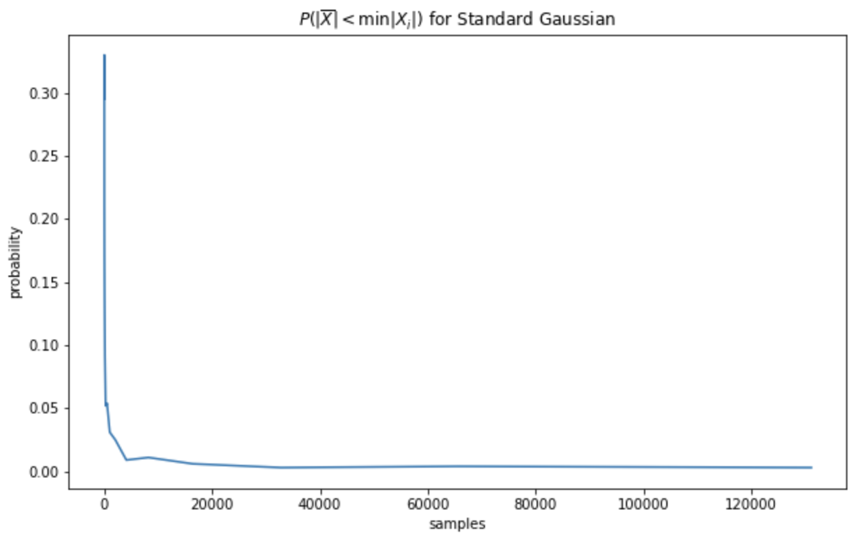
It seems pretty convincing then that the probability of winning actually converges to 0 as $n \to \infty$ so the rate at which the best guess converges is faster than the rate at which the sample mean converges to the true mean.

Relative Ranking in the Jelly Bean Game

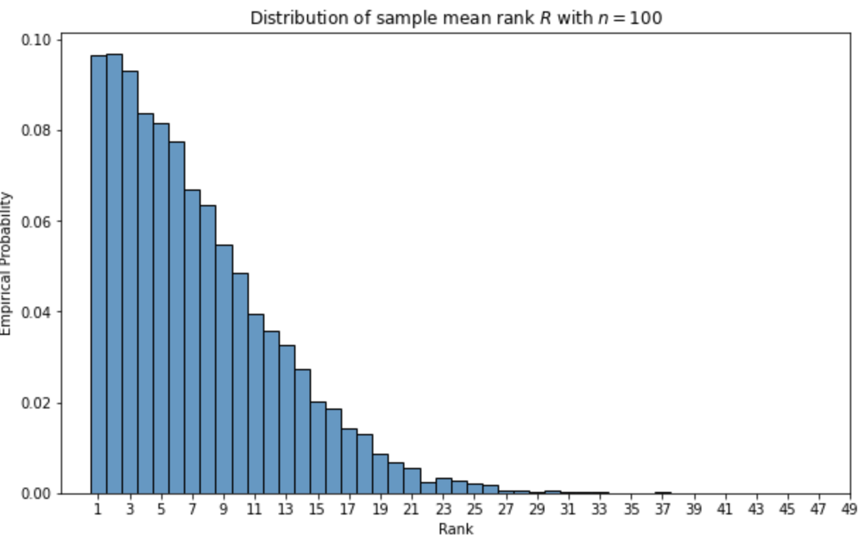
The next line of questioning is where does our sample mean rank $R$ amongst the other guesses. Can we almost surely be, for any value of $0 < q \leq 100$, in the top $q$ percentile for sufficiently large $n$? Can we be in the top $O(n^{-r})$ percentile for some value of $r > 0$? Empirically sampling the distribution of $R$ given $n = 100$ shows us that the distribution of rank looks roughly half-normal with mean rank $7.28$

We can sample the rank distribution for various values of $n$ to view $\mathbb E[R]$ as a function of $n$. Here it is plotted alongside the function $f(n) = 0.64 \sqrt{n}$

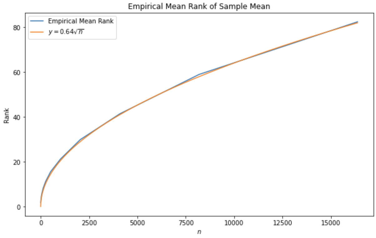
It seems clear that your expected rank in the jellybean contest if you submit the sample mean is $O(\sqrt{n})$. This means, in particular, that as $n \to \infty$, you can almost surely be in the top $q$ percentile for any $q > 0$. A proof of this follows from markov's inequality: \[\begin{aligned} \lim_{n \to \infty} \mathbb P[R \geq qn] &\leq \lim_{n \to \infty} \frac{\mathbb E[R]}{qn} \\ &= \lim_{n \to \infty} \frac{1}{q} O(n^{-1/2}) \\ &= 0 \end{aligned} \] Which implies that $\lim_{n \to \infty} \mathbb P[R \leq qn] = 1$.s A stronger result is that for any $r < 0.5$, you can almost surely be in the top $O(n^{-r})$ percentile, the proof of which follows identically: \[\begin{aligned} \lim_{n \to \infty} \mathbb P[R \geq O(n^{-r})n] &\leq \lim_{n \to \infty} \frac{\mathbb E[R]}{qn} \\ &= \lim_{n \to \infty} \frac{1}{q} O(n^{r-1/2}) \\ &= 0 \end{aligned} \]

Higher Dimensional Cases

Something peculiar happens when we consider high dimensional cases. What if participants have to submit multiple guesses? Suppose that in addition to guessing the number of jelly beans in a jar, they have to submit a guess for the combined total number of pets owned by everyone at the school. It is reasonable to assume that people's guesses for these are fairly independent (i.e. if you told me someone guessed that there are $x$ jelly beans, it gives me little information about how many pets they guessed). We can then model the joint distribution of guesses for each participant \[ \begin{aligned} X_i \overset{\text{i.i.d}}{\sim} \mathcal N(\mu, \Sigma) = \mathcal N(\begin{bmatrix} \mu_1 \\ \mu_2 \end{bmatrix}, \begin{bmatrix} \sigma_1^2 & 0 \\ 0 & \sigma_2^2 \end{bmatrix}) \end{aligned} \] Here, $\mu$ is now a vector in $\mathbb R^2$ and $\Sigma$ is a matrix in $R^{2\times 2}$. $\mu$ has components $\mu_1$ and $\mu_2$ where $\mu_1$ is the true number of jelly beans and $\mu_2$ is the true number of pets. $\Sigma$ is a diagonal covariance matrix (since we are assuming independence) in $\mathbb R^{2 \times 2}$ with diagonal components $\sigma_1^2$, the variance associated with the jelly bean guesses, and $\sigma_2^2$, the variance associated with the pet guesses. Then, for some distance metric $d : \mathbb R^2 \times \mathbb R^2 \to \mathbb R$, the sample mean wins if: \[\begin{aligned} d(\overline{X}, \mu) < \min_{i} d(X_i, \mu) \end{aligned} \] If $d$ is translation invariant, such as in the case where $d$ is an induced metric of a normed vector space $d(x,y) = \|x - y\|$, consider the transformed variable \[ Y_i = f(X_i) = \Sigma^{-1}(X_i - \mu) \] Equivalently we win if \[ \begin{aligned} &d \Bigg( \Sigma \Big (\sum_{i=1}^{n} \frac{1}{n} Y_i \Big) + \mu , \mu\Bigg) < \min_{i} d(\Sigma Y_i + \mu, \mu) \\ \equiv ~& \big \| \Sigma \overline{Y} \big \| < \min_{i} \big \| \Sigma Y_i \big \| \end{aligned} \] In the special case where our variances for each estimate are equal (i.e. $\Sigma = \sigma I$), winning is equivalent to the condition \[ \|\overline{Y}\| < \min_{i} \|Y_i\| \] This problem is much nicer to look at because it does not depend on $\mu$ or $\Sigma$ since $Y_i \overset{\text{i.i.d}}{\sim} \mathcal N(0, I)$ and $\overline{Y} \sim \mathcal N(0, 1/n I)$.

We will only consider the case where all variances are equal because the case where one estimate is much noisier than the other reduces the problem to the one-dimensional case (intuitively, if one quantity is known, the problem of finding the best guess across two unknown quantities is the same as finding the best guess across one unknown quantity). This method works for any finite number of estimates, with the dimension of our space corresponding to the number of estimates. We have in addition proven in full generality that any norm will be satisfiable. For our purposes, we will only consider the $\ell_2$ norm although I suspect the results will be equivalent (down to some constant factor perhaps) for any $\ell_p$ norm.

In what follows, I only have empirical results. The math in higher dimensional cases are almost certainly less tenable to analytic solutions than the one dimensional case. But still, I think the empirical results are fascinating and leave me with a few conjectures I will list at the bottom of this post. To begin win, let's look at the probability of winning the game in the case of the two-dimensional and three-dimensional game.

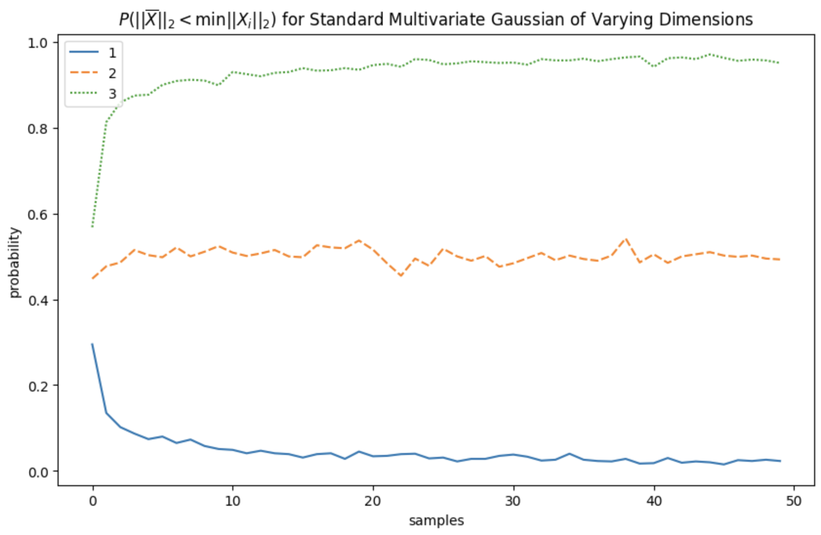
Our empirical measure of the true probability is noisy since we're estimating it 1000 samples. Without proving so statistically, this graph seems to suggest that the true probability of winning does not depend on $n$ and is a constant 0.5. This is rather striking as it suggests that playing the game with two independent equal-variance estimates gives you a probability of winning equivalent to flipping a coin, and your decision to participate should be independent of the number of other participants. As you might expect then, in the three-dimensional case, the probability of winning converges to 1 as $n \to \infty$. It would seem that two dimensions is the tipping point, below which we asymptotically expect to lose and above which we can asymptotically expect to win. What is most interesting is that the tipping point lies exactly at the two-dimensional case, where we have a non-zero probability of both winning and losing. The next course of action is to analyze the expected relative ranking in the game as a function of $n$.

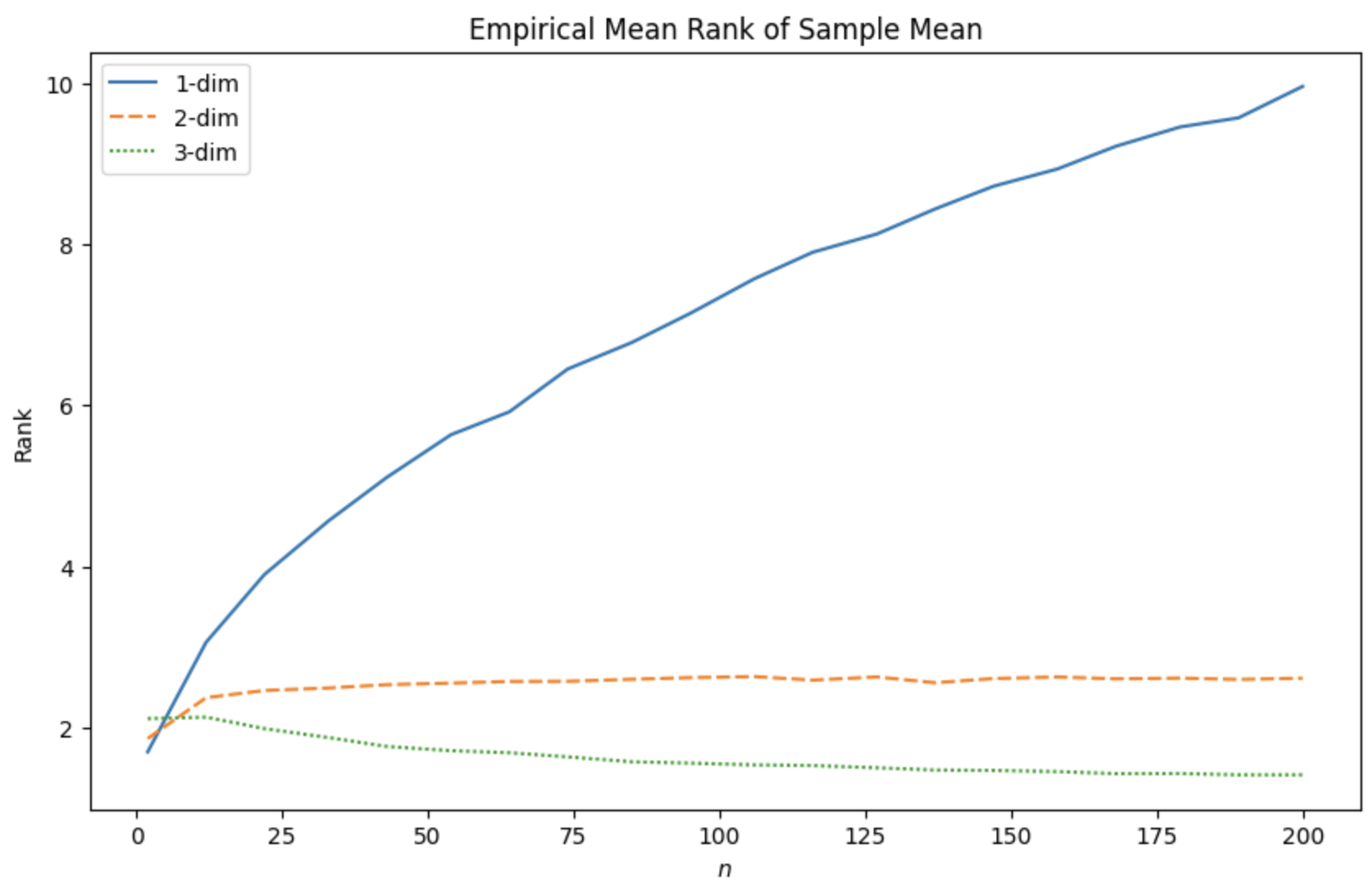
For $d=2$, as will our probability of winning, our expected rank doesn't depend on the number of people playing. Which is a bit counterintuitive since that means we are on average ~2.6th place regardless of how many contestants there are. For $d = 3$, not only do we probabilistically converge to winning, but in expectation our rank also converges to $1$, which follows our intuition since we don't expect the variance to grow too fast.

Conjectures

For the things I was only able to study empirically, I have some analytical hypotheses that I would conjecture extend to even higher dimensions:

1. The rank distribution in the $d=1$ case approaches a discretized half-normal distribution as $n \to \infty$. That is, on a support of $[0, \infty)$, $\mathbb P[R = k] \propto e^{-ck^2}$ where $c$ could depend on $n$. For higher dimensions, I believe the distribution is subgaussian where $\mathbb P[R = k] \propto e^{-ck^{2/d}}$. In particular, this suggests the distribution for $d=2$ is geometric.

2. The asymptotic mean rank for the $d=1$ case is $\Theta(\sqrt{n})$. For arbitrary dimension, the asymptotic mean rank is $\Theta(n^{1-d/2)})$

3. Conducting the above analysis on any $\ell_p$ metric would yield the same asymptotic bounds